Playing with Vision Embeddings
Corn kernels
Arc de Triomphe
Arc de Kernel
Embeddings are, in a sense, the native language of neural networks. They are how networks can encode a rich variety of semantically meaningful representations with just a list of numbers. However, those numbers are frustratingly opaque, you certainly won't be able to make sense of them by reading them one after another. In this post, we try to make sense of one neural network's embeddings.
The Model
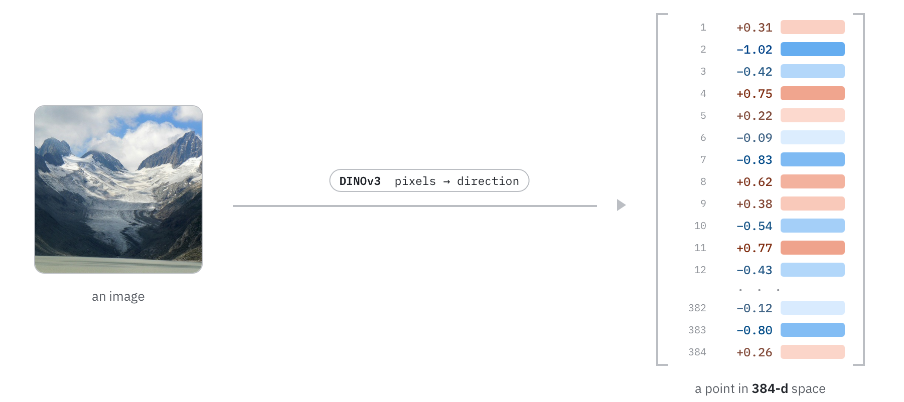
The model we're going to be looking at in this post is DINOv3 ViT-S (Siméoni et al., 2025). DINOv3 is interesting because it learns to map raw pixels to a rich feature space with very few priors. It doesn't know language, it can't describe what it sees, but it still learns to make sense of images. We won't go into detail about how DINOv3 was trained, but the important thing to know in this post is that it compresses any image into a single embedding. This embedding is a list of 384 numbers and our goal is to understand what information is encoded in those 384 numbers.
Generating Images from Embeddings
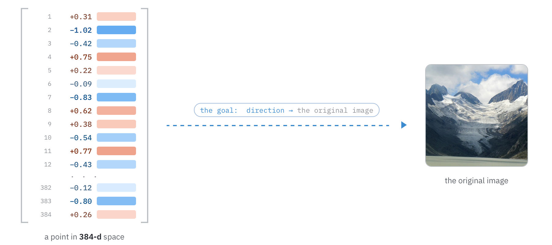
In order to start playing around in this 384-dimensional space, we need some way to translate these numbers back into something that humans can understand. The most natural place to do this is in the one language humans and DINOv3 both understand: images. More concretely, we want to be able to take a point in this 384-dimensional space and generate an image that DINOv3 says would coincide with that point.
To do this, we leverage two ideas: the first is that DINOv3 is fully differentiable -- when you feed an image into the model, you can tweak the pixels to make the output vector closer to some target. The second is that DINOv3 was trained such that different crops and augmentations of an image will land in the same embedding space. There are a couple other tricks we do to make the images look nicer, such as using an untrained transformer backbone to produce the image, and minimizing an auxiliary total variation loss.
Once this pipeline is set up, when given an arbitrary direction in 384-dimensional space, we can generate an image that DINOv3 says would point in that direction. For example, below we take a photo of an alpine landscape, compute its DINOv3 embedding, and then use our generation technique to produce an image that points in that same direction.
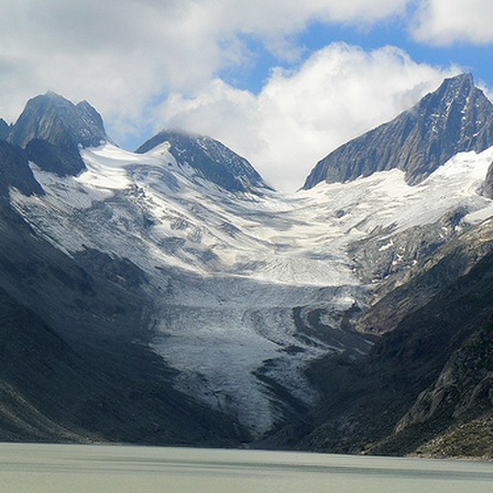
Original

Raw pixels no augmentations

Raw pixels with augmentations

Transformer with augmentations
Now, the generated image seems to capture the general vibe of the original image, it clearly shows mountains, snow, and a lake. Take a look at the spread of images generated to get a fuller sense of what's generated:
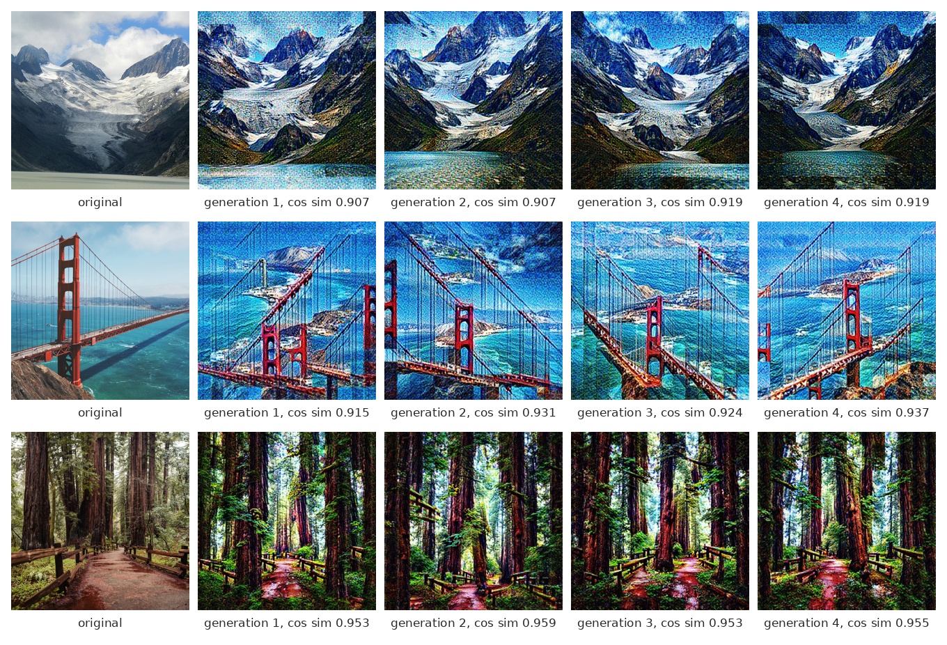
You'll see some variation generation to generation (after all, we are compressing an entire image down to 384 numbers, which is inherently a many-to-one operation). But you'll also notice that there are a few common ways that they differ from the original. They're more saturated, higher contrast, and they misplace/duplicate some of the objects in the scene. Most of this is likely due to the generation pipeline itself, as hinted at by their cosine similarities to the original being ~0.9, but it could also partly be how the model sees things. It's hard to tell whether it's the instrument or the subject sometimes.
Finding the features
The first thing we need to understand before we start trying to pick apart the 384-dimensional space is that DINOv3 encodes far more than 384 distinct visual concepts into those 384 numbers. How? The leading hypothesis is something called superposition: models learn to cram many times more features than the dimensionality of their embeddings by pointing each feature in a nearly-orthogonal direction (Elhage et al., 2022).
To demonstrate this phenomenon, we'll show how a small toy neural network can squeeze 10 MNIST digit classes through a 2-dimensional bottleneck. Every frame here corresponds to one step by the optimizer so you can see the model learn to represent all 10 classes.
10 digit classes squeezed into 2 dimensions. Each class gets its own slanted direction.
The key observation is that neural networks tend to place features along directions in their hidden space. Each of those 10 digit clusters above appears to point in distinct directions out from the origin. In 2 dimensions there's room for maybe 10 before they start stepping on each other, but in 384 dimensions there's room for thousands.
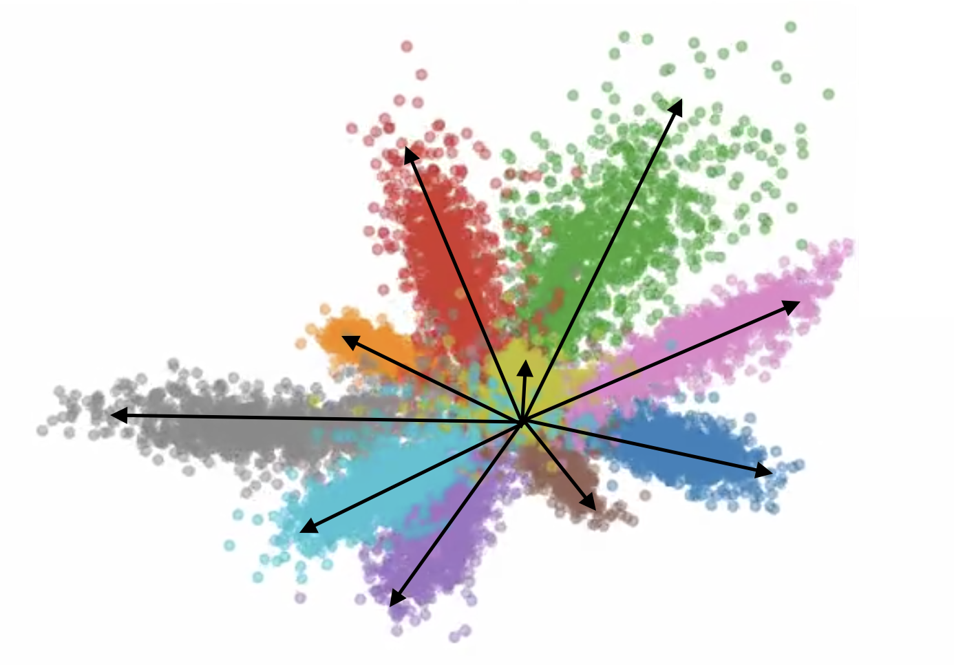
The same 10 clusters, annotated with the feature direction each one points along.
Superposition is a double-edged sword. On the one hand, it allows models to learn many times more features than they have dimensions. On the other hand, it means that any single dimension of DINOv3's embedding is a smear across many concepts at once, which makes it hard to understand directly.
To pull the concepts back apart into individual, interpretable directions, one tool at our disposal is to train a sparse autoencoder (SAE). The idea is first to give the model's representations more room to breathe. We do this with a simple linear mapping from the model's 384-dimensional feature space to a much higher 12,288-dimensional space.
What we want is for each of those 12,288 dimensions to correspond to a single unique feature. To do this, we need some method to penalize feature smearing (or equivalently to incentivize sparsity). We do this with an L1 sparsity penalty on the 12,288-dimensional representations. Finally, we try to reconstruct the original embeddings given only the high dimensional sparse features, giving us a training objective. Each feature is a direction in the embedding space. There are a few other optimizations and improvements we use for our demonstration here, but this is the core idea.[1]
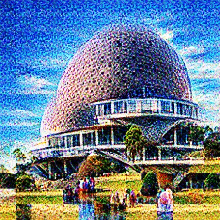
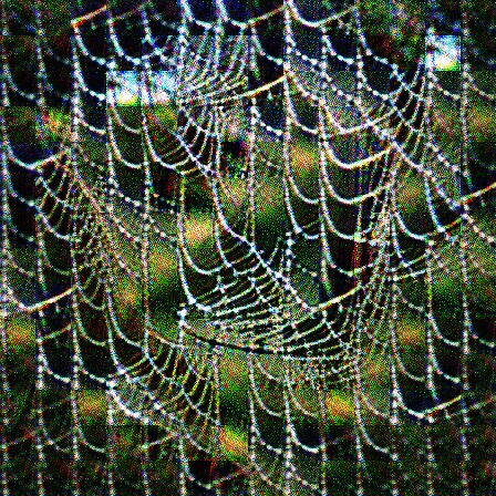
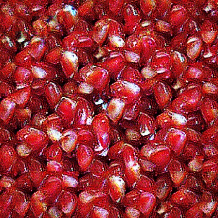
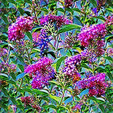
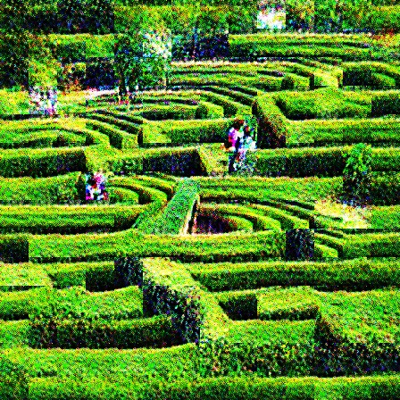
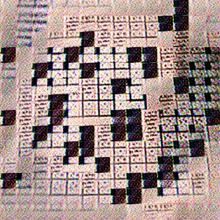
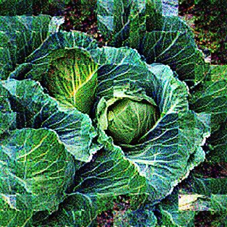
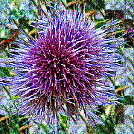
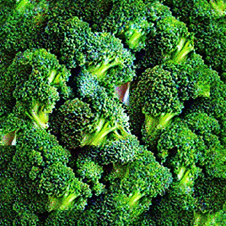
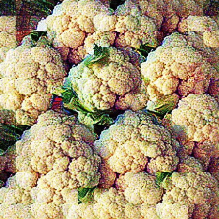
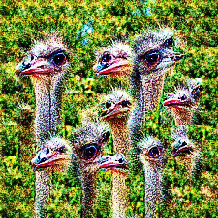
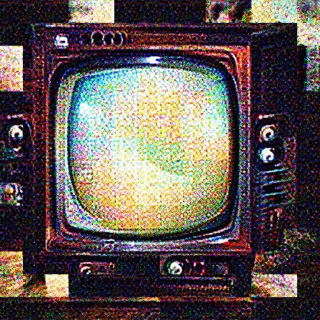
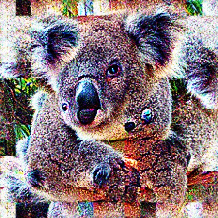
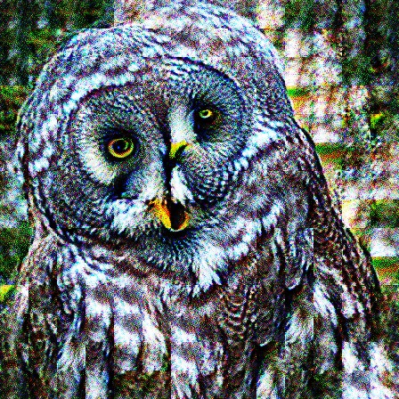
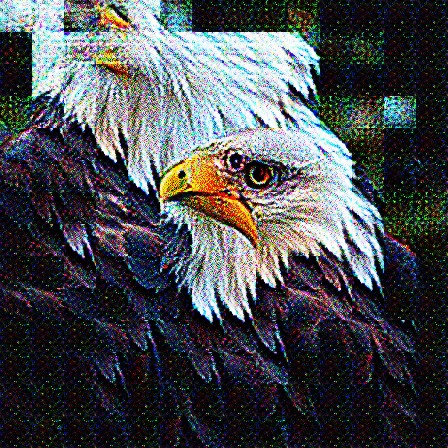
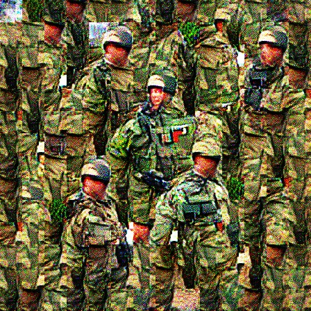
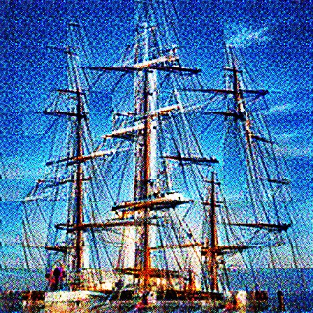
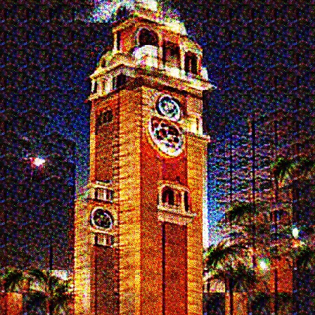
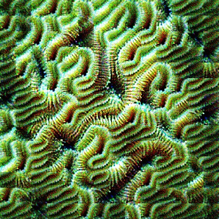
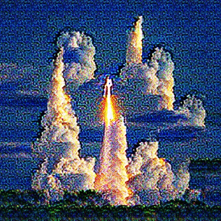
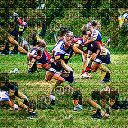
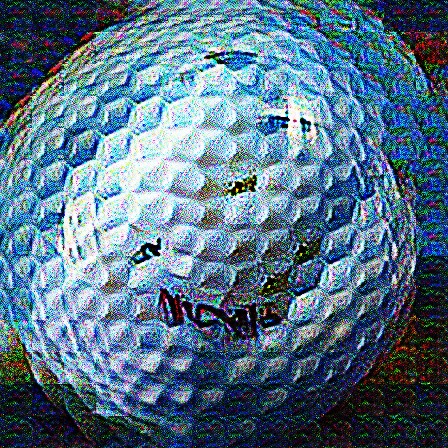
Once trained, we can run our learned features through our image generation process and see what they represent. We show a handful here (or you can browse all features in a separate tab →). Click on any image to expand it, many have intricate details that are easy to miss when they're small.





Decomposition
The SAE is a powerful tool. The most straightforward thing we can do with it is to decompose a given embedding into a set of the learned sparse features, effectively giving us a tool to see what kinds of features the model is encoding within an embedding.
Below, we feed in a photo of a redwood forest path, take its DINOv3 embedding, and run it through the SAE. The features that fire most strongly are shown beneath the photo, sorted by activation strength. The blue bar under each tile shows how strongly that feature fires.
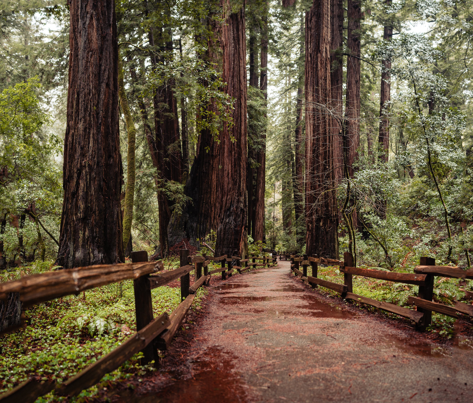
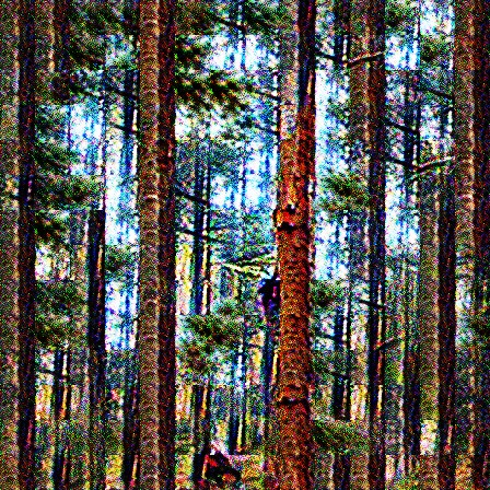
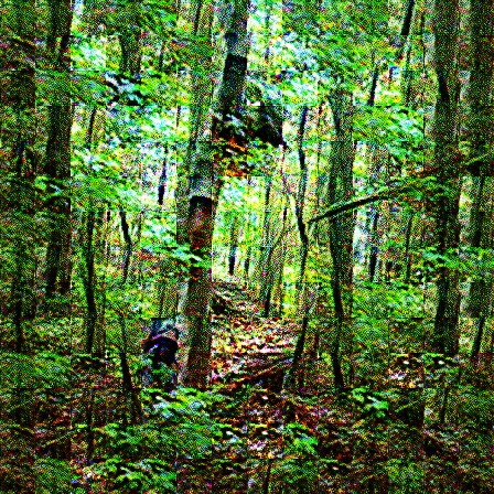
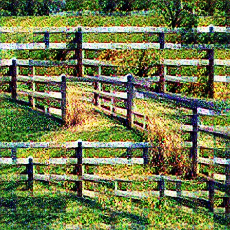
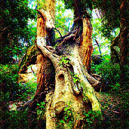
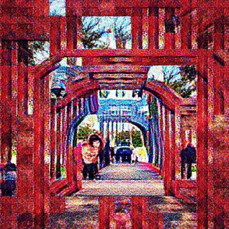
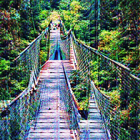
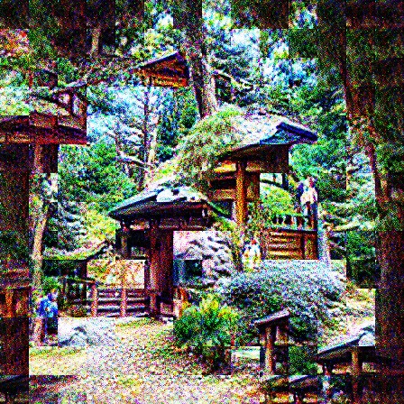
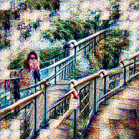
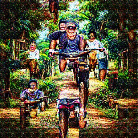
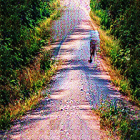
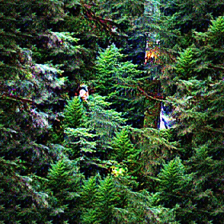
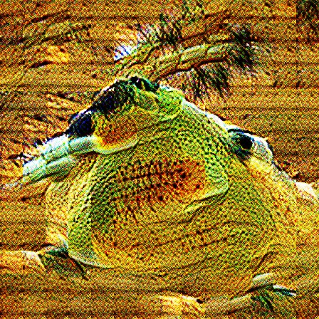
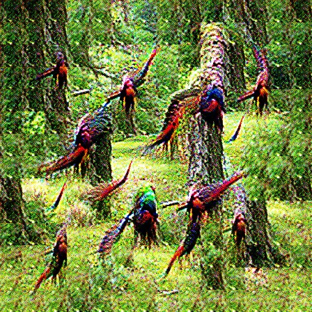
The features that activate for this photo are all pretty clear -- trees, greenery, fences, paths. It's a decomposition of the image into its component features.
We can do the same thing for an image of the Golden Gate Bridge:

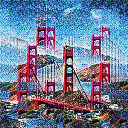
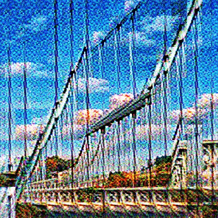



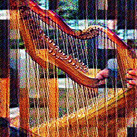


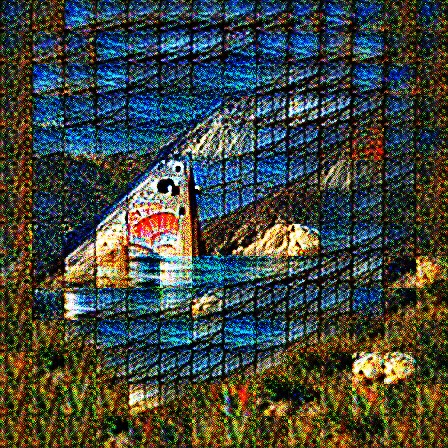
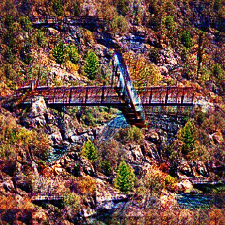
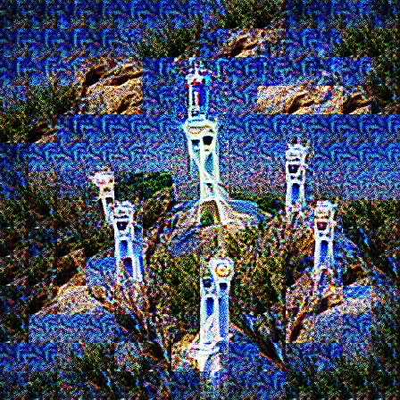
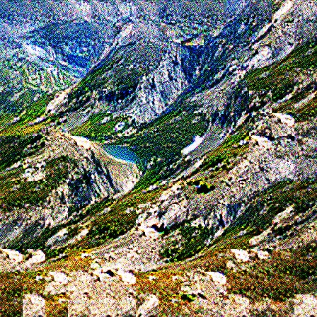


What's interesting about this one is that the strongest feature appears to be a feature dedicated specifically to the Golden Gate Bridge itself. Keep in mind, this is only a 22M parameter model! Having a feature dedicated to this at this size is impressive. Claude 3 Sonnet would approve.
Addition
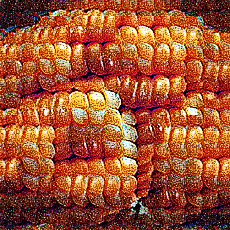
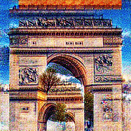
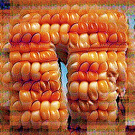
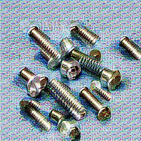
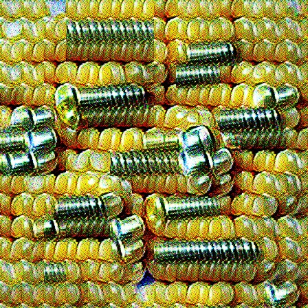
One of the assumptions in our training of the SAE is that different features can be added together to create another reasonable embedding. Here, we're going to play with this assumption directly. We pick two feature directions, sum them together to produce a new direction, and run our generation technique on that direction to see what it produces. For example, corn kernels plus the Arc de Triomphe, or corn kernels plus screws:
Corn kernels
Arc de Triomphe
Arc de Kernel
Corn kernels
Screws
Screws on corn
The result isn't a pixel-level average between the two component features, but something a little stranger. In the corn/arch example, the combined direction is a fusion, it generates the Arc de Triomphe out of corn. With the corn/screws example, it's more of a juxtaposition, it puts screws on top of the corn.
Most additions aren't as clear cut as these two, usually the additions are somewhere between a fusion and juxtaposition. See for yourself by adding any of these together:
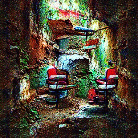

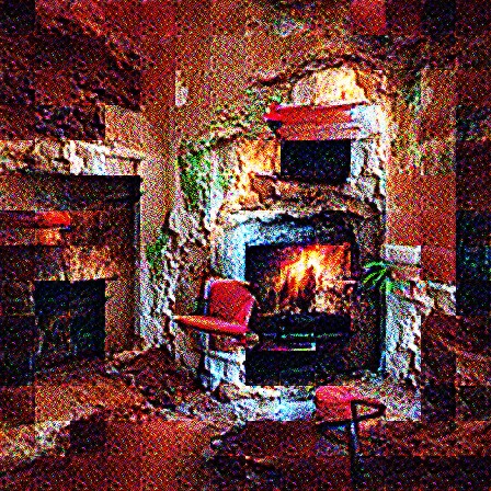
It's not clear why features added together merge the ways they do. It might have to do with the sparsity of the features; adding two features that never fire together might just merge together in strange ways. It might also be that some features encode textures while others encode structure. It's hard to tell with just these tools.
Two Strawberries
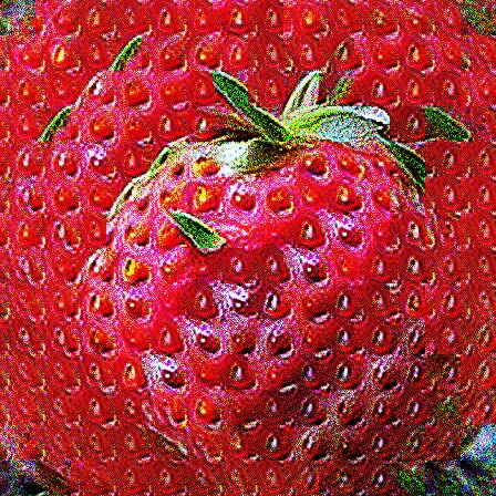
In going through the SAE features, I found two features that looked to both be about strawberries. In this section we're going to dive deep into these two strawberry features and try to determine concretely what each of them actually encodes.
feature 1511
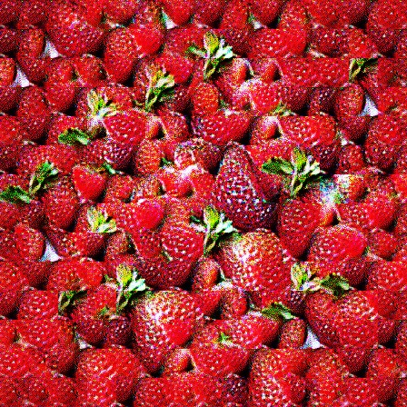
feature 2314
Just looking at them, it seems like the first one (feature 1511) is encoding a singular strawberry and the second (feature 2314) is about a group of many strawberries. We can amplify their differences by stripping out the directions that they share to get a better look at what distinguishes them. This process is called Gram-Schmidt orthogonalization, and this is what the result looks like:
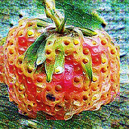
1511 ⊥ 2314
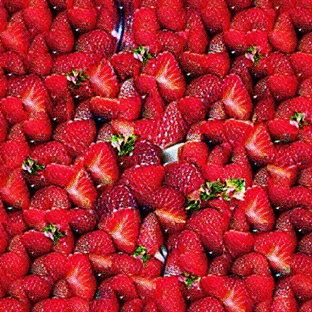
2314 ⊥ 1511
This definitely strengthens the case that 1511 really is encoding a single whole strawberry, complete with all its seeds and the top, and 2314 is encoding many strawberries, even if they're cut open. But is 1511 about being a single strawberry? Or about being a whole strawberry? And is 2314 about being many strawberries? Or about being small strawberries?
To try to pick this apart, we'll start by feeding into our SAE an image of a strawberry at different sizes and record the strength of both of our features as we scale. Use the slider below:
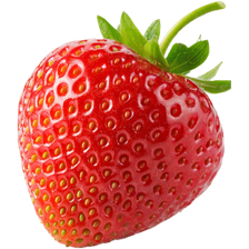
224×224 px
Looking at the graph above, the story is pretty clear. The bigger the strawberry is, the stronger 1511 activates. The smaller it is, the more 2314 activates (until the strawberry is roughly ~30x30 pixels, at which point it starts to go down again).
Now, let's try to see if the number of strawberries matters too. We'll keep the size of the strawberries at 125x125 pixels, which was solidly in the 1511 territory in the size experiment.
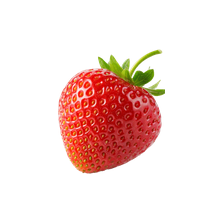
1 strawberry
So it seems that the number of strawberries is also part of what distinguishes 1511 and 2314, independent of the size of the strawberries. More strawberries -> higher 2314 and lower 1511.
Now, one final check to see if we understand everything correctly. To get a baseline, this is how much 1511 and 2314 activate for a single, large, whole strawberry:
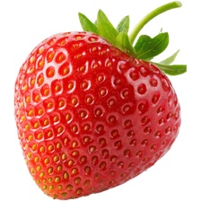
one large whole strawberry
As expected, feature 1511 dominates. Now, what will we see for a single, large, sliced strawberry?
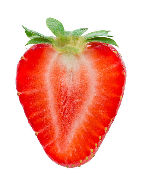
one large sliced strawberry
1511 collapses! This means that 1511 is a feature specifically for single, large, whole strawberries, and 2314 is about many small strawberries whether whole or sliced.
Hopefully this gives you an idea of how intricate and nuanced each feature is. We only looked at two in depth here, but our SAE generated twelve thousand. Interpreting all of them is incredibly difficult, and doing a manual analysis is not scalable.
The Map
To wrap up, we'll zoom out and look at what the whole feature space looks like. We ran the SAE across a large image corpus (ImageNet Val) and recorded, for every image, the set of features activated. This gives us a large coactivation matrix for the features which we can use with UMAP (McInnes et al., 2018) to visualize the large feature space in 2 dimensions while preserving local neighborhoods, so features that often activate together land near each other on the map. This is similar in spirit to the activation atlases of Carter et al. (2019). Scroll around and zoom in/out to see the different features and clusters the SAE learned:
Drag or swipe to pan · scroll or pinch to zoom · 2500 of the strongest features on an 120×120 grid
What This Means
One thing that sits with me after all of this is that it's really difficult to understand how neural networks encode information. DINOv3 was trained without labels, we generated features from its embeddings without labels, and now we've gone through and tried to make sense of some of those features, attempting to label them in natural language. And it takes a lot of work. It's like doing neuroscience on an alien brain with alien tools.
[1] We trained the SAE on DINOv3 ViT-S/16 global (CLS) embeddings: a 32× expansion (384 → 12,288) with ReLU activations and an L1 sparsity penalty, with periodic resampling of dead features (Bricken et al., 2023). At inference we keep only the top 32 features active per image.